False vacuum decay 2.0
I would like to tell you about my latest paper: “Non-perturbative methods for false vacuum decay”, co-authored with Eleanor Hall and Hitoshi Murayama from Berkeley.
I wrote about false vacuum decay some time ago. Back then, I promised to write a series of post about doomsday scenarios; but I did not deliver on that promise. Instead, I can recommend a recent book about this very topic.
Gravitational waves from the early Universe
In this new work, we propose a new (non-perturbative) technique to calculate false vacuum decay rates. It is important to calculate this rate accurately, because it is needed to forecast the spectrum of gravitational waves from the early Universe.
You see, unlike other signals (like photons and neutrinos), gravitational waves can in principle be used to study the first second of the Universe. There are many candidate-theories for that cosmological period which can be distinguished using gravitational waves. These theories feature a first order phase transition: a phase transition with false vacuum decay.
The challenge
Unfortunately, accurately calculating the gravitational wave spectrum from a first order phase transition is a big challenge. Existing methods struggle particularly with strong couplings. Why?
The effective action — physics-speak for “the thing that describes the dynamics of the theory” — is by definition convex. Here’s an illustration of what that means:
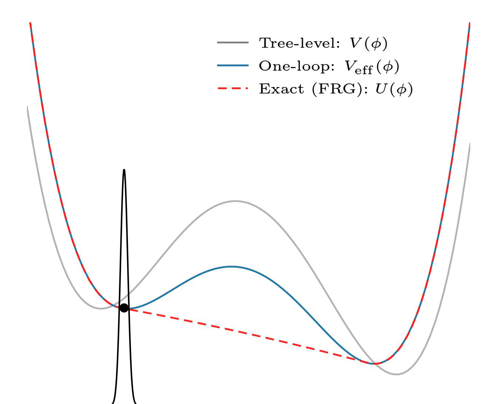
Illustratration of convexity, by my collaborator Eleanor Hall. Note the red-dashed line. Convexity means something like “only has a single minimum”. It is realized by states with field value between two mimima in the potential (in grey) by forming a superposition of the two minima (check out this classic paper by E. Weinberg and Wu).
But that is a problem! After all, false vacuum decay requires a false vacuum. This cannot be the effective action we are looking for.
The perturbative solution
An often-employed solution to this problem is perturbative: it uses and relies on the fact that there is a small parameter (the coupling constant). Here is an example:
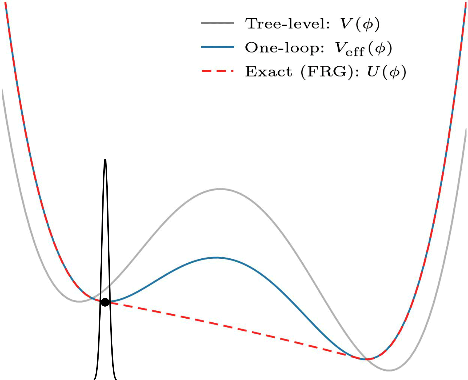
Non-convexity of the one-loop effective potential. In this perturbative approximation, coarse graining ensures no superpositions, and convexity is not necessary. This one is also by my collaborator Eleanor Hall.
This is all fine for theories which have a small coupling, but what about the ones that do not? Some of these need studying too! (And there are some other issues that I will spare you.)
A non-perturbative proposal
We propose an alternative, where we explicitly enforce locality in field space. This means that the superpositions above do not happen. Here is an illustration:
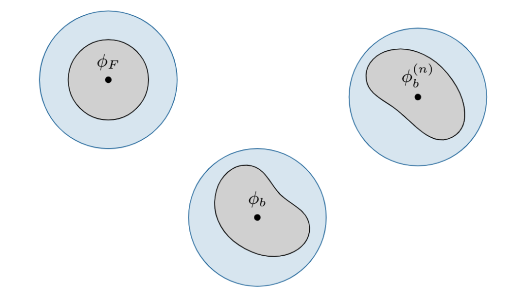
We only consider the important blue blobs.
We also show how to do this: it is possible within the framework of functional renormalization. That is a super impressive framework developed over the last few decades.
A simple example
In this first paper we also worked out a simple example, which we compare to the result found in other methods. As expected, the difference creep in at stronger coupling:
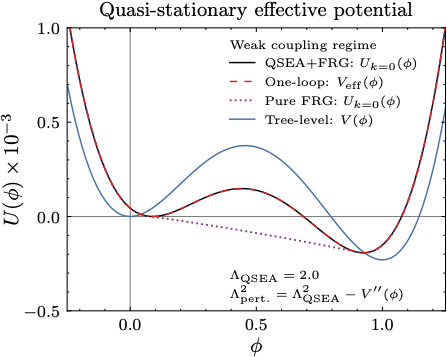
Our proposal (black continuous lines), compared to other methods. In the weak coupling regime (small coupling constants) the results are the same as in perturbation theory (red dashed lines)…
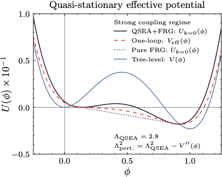
…but in the strong coupling regime the predictions are different, as expected.
That’s it! We are excited that our proposal matches the old results where we expect it to, and diverges where we do not.
We hope to develop the method much further. Eventually, we want to study things like confinement / chiral symmetry breaking (in theories beyond the Standard Model) — and calculate the resulting gravitational wave spectra. I can’t wait to learn more.